Impact Factor ISSN: 1449-2288
- Issue 12; 2026
- Issue 11; 2026
- Issue 10; 2026
- Issue 9; 2026
- Issue 8; 2026
- Volume 22; 2026
- Past Issues
- Advance Articles
- Editorial Board
- Cover Images
- Index & Coverage
- Cover Suggestion
- Special Issues
Introduction
Lung sound recognition process
Wavelet transform, LDA and BP...
Wavelet decomposition and...
Experiment with BP neural network
Conclusion
Acknowledgements
References

 Global reach, higher impact
Int J Biol Sci 2019; 15(1):195-207. doi:10.7150/ijbs.29863 This issue Cite
Research Paper
A Lung Sound Category Recognition Method Based on Wavelet Decomposition and BP Neural Network
Yan Shi1 ![]() , Yuqian Li1, Maolin Cai2, Xiaohua Douglas Zhang2
, Yuqian Li1, Maolin Cai2, Xiaohua Douglas Zhang2
1. School of Automation Science and Electrical Engineering, Beihang University, Beijing 100191, P.R. China
2. Faculty of Health Sciences, University of Macau, Taipa, Macau.
Received 2018-9-11; Accepted 2018-10-15; Published 2019-1-1
Abstract

In this paper, a method of characteristic extraction and recognition on lung sounds is given. Wavelet de-noised method is adopted to reduce noise of collected lung sounds and extract wavelet characteristic coefficients of the de-noised lung sounds by wavelet decomposition. Considering the problem that lung sounds characteristic vectors are of high dimensions after wavelet decomposition and reconstruction, a new method is proposed to transform the characteristic vectors from reconstructed signals into reconstructed signal energy. In addition, we use linear discriminant analysis (LDA) to reduce the dimension of characteristic vectors for comparison in order to obtain a more efficient way for recognition. Finally, we use BP neural network to carry out lung sounds recognition where comparatively high-dimensional characteristic vectors and low- dimensional vectors are set as input and lung sounds categories as output with a recognition accuracy of 82.5% and 92.5%.
Keywords: lung sound, category recognition, wavelet de-noising, linear discriminant analysis, BP neural network
Introduction
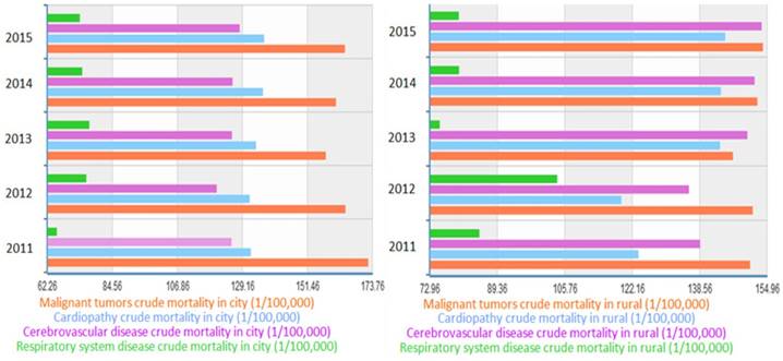
In recent years, the incidence of respiratory system diseases such as chronic obstructive pulmonary disease, bronchitis and asthma tend to rise gradually due to the atmosphere contamination, for instance, frequent haze [1]. Respiratory disease is now listed as one of the leading causes of death of domestic residents according to statistics from the National Health Bureau [2]. In 2015, the death rate due to respiratory system diseases was 7.336 and 7.996 per one thousand people among urban and rural domestic residents respectively [3]. Figure 1 is the crude death rates caused by some main diseases in domestic city and rural, which indicates that the respiratory disease is non-negligible and noteworthy. It is meaningful to research on lung diseases to prevent death and promote treatment and clinical level [4,5].
Crude death rates of diseases in city and rural
With the increasing incidence of respiratory system diseases [6], more attention is being paid on the harmless diagnosis method based on analysis of lung sounds which contains abundant information on lung condition. However, conventional auscultation of lung sounds has a very limited usage because of the limitation of information it can obtain, its dependence on physician's experience, and its high rate of misdiagnosis. Therefore, it will be helpful to develop an efficient method to recognize lung sounds and to diagnose related diseases based on the analysis of the more informative lung sounds data collected by electronic stethoscope and develop an efficient way to recognize lung sounds and its related diseases [7,8]. During diagnosis process, it is helpful for accurately judging characteristic vectors and determining disease reasons to de-noise lung sounds and abstract vibration frequency, sound waves amplitude and amplitude gradient [9-12].
The classification of lung sounds could be dated back in 1819 when Leannec published Indirect Auscultation sorting it into five kinds. With more researches on its classification there came various supplement and modification on lung sound categories [13-19]. Taking health condition into consideration, lung sounds are mainly classified into three types: normal, abnormal and adventitious [20,21]. Normal lung sound is mainly generated from the airflow through principle bronchi, bronchiole and lung in the respiratory system [22]. The abnormal and the adventitious lung sounds are produced when there exist problems or something unfit in human body. Table 1 shows the lung sound categories in detail [23].
Lung sound categories
| Lung Sounds | ||
|---|---|---|
| Normal | Vesicular sound, tracheal sound, bronchial sound | |
| Abnormal | Weaken, vanished sound, prolongement expiratoire, tubular breathing sound | |
| Adventitious | Coarse crackles | Discontinuous sound (Moist rale) |
| Fine crackles | ||
| Wheezes | Continuous sound (Dry rale) | |
| Rhnochus | ||
| Others | Chest rubs, etc. | |
The normal lung sounds primarily include three categories: vesicular breathing sound, bronchial breathing sound and tracheal sound. The abnormal lung sounds consists of weaken and vanished sound, prolongement expiratoire and tubular breathing sound. In 1985, adventitious sounds, a kind of additional noise in periodic signal [24], was principally identified by The 10th International Respiratory Voice Association as: coarse crackle, fine crackle, wheeze, and rhonchus. Coarse crackle is discontinuous sound called moist rale while the others are continuous sound called dry rale. There are also some other lung sounds, chest rubs for instance.
For a long time there have been a lot of researches on lung sounds and its pathologic causes [25-27]. The common coarse crackles in patients with pulmonary interstitial fibrosis, bronchiectasis and chronic bronchitis last for about 5s [7,28]. Coarse crackles symptoms are shown as inflammation, such as pneumonia, pulmonary congestion, early pulmonary edema, bronchitis, alveolar inflammation and other diseases. Wheeze is usually associated with chronic obstructive pulmonary disease such as bronchial asthma and cystic fibrosis. Rhnochus with the frequency about 200Hz or below is mainly caused by bronchitis [29,30]. Certainly accurate judgment of pathological features is also limited by subjective factors from auscultation physicians and passive factors from patients [31,32]. It is possible to provide efficient method for lung sounds analysis through frequency analysis [33].
Yao et al. combined with wavelet analysis and genetic neural network method for statistical characteristic extraction and classifier design to distinguish lung sounds category whose recognition accuracy was 89% [29]. Through wavelet packet transformation, Lee et al. improved recognition accuracy of lung sounds in high frequency ranges and improved detection and analysis accuracy of lung sounds [34].
Considering the significance of research on lung sounds, we summarize lung sounds categories and their related diseases. In addition, it is more efficient for lung sounds analysis through frequency analysis because that accurate clinic judgment is limited by subjective factors from auscultation physicians and passive factors from patients. In this paper, we use wavelet transform to decompose lung sounds and identify lung sounds (dry rale and moist rale) according to characterization of lung diseases.
The rest of this paper is organized as follows. Section 2 briefly introduces the whole process of lung sound recognition in this study. Section 3 introduces the basic principle of wavelet transform, linear discriminant and BP neural network, which are used in the lung sound recognition process. In Section 4, we use wavelet transform to decompose lung sounds and linear discriminant to reduce space dimension so that appropriate vectors can be gotten for the process of recognition. In section 5, experiment based on BP neural network are tried to identify lung sounds (dry rales and moist rale) according to characterization of lung diseases, and the recognition accuracy of the data after LDA can reach 92.5%. Finally, we conclude the paper in Section 6 by summarizing the process of the algorithm and proving the validity by comparing the result with other researchers.
Lung sound recognition process
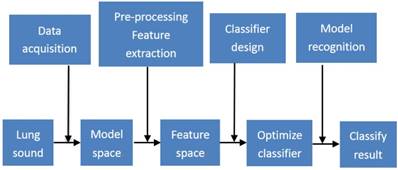
In the early days of lung sound researches, acquisition technology was the key focus, pneumatic sensor for instance [35]. With the development of computer and electronic, lung sounds could be recorded and change its form from analog signal to digital signal. Electronic stethoscope is popular these years for its advantage of high sensitivity, high magnification, superior resistance to distortion and simple analysis [36]. Bluetooth technologies can achieve recording data transmitting to computer in real-time, sharing specialist consultation online for remote diagnosis. Figure 2 is lung sound processing structure diagram in whole composed by data acquisition, lung sound acquisition, pre-processing, and characteristic extraction, classify design and model recognition. The lung sounds collection part is consist of 3M electronic stethoscope and detecting lung sounds in lung and other organ location could achieve lung sounds collection. Then using wavelet de-noising and wavelet transform could extract characteristic values. Through transforming reconstructed signals and linear discriminant analysis, it is helpful to reduce characteristic vector dimension for better recognition effect. Finally we deal with lung sounds recognition through BP neural network.
Lung sound processing structure diagram
Wavelet transform, LDA and BP neural network
Wavelet transform
Wavelet transform is a new transform analysis method. It inherits and develops localization idea of short-time Fourier transform and overcomes the shortcomings, the window size does not change when frequency changes while wavelet transform could provide the changeable time-frequency window for instance. While wavelet transform could guarantee the resolution of frequency domain in the high-frequency band and the resolution of time domain in the low-frequency band with the changeable time-frequency window. This means a multi-resolution method allowing for the coarse to precise resolution in frequency and time domain can be used in this research, which provides enough information of the lung sound signal. Main feature of wavelet transform is that it could fully highlight characteristics of certain aspects and analyze localization of frequency. Time subdivision in high-frequency and time coarse-division in low-frequency could be achieved through extend-shift operation of signal, which could automatically adapt to requirements of time-frequency signal analysis and focus on any signal details.
For integrable signal f(x), its continuous wavelet transform is shown as formulas (1) and (2) with energy conservation of base functions shown as formula (3):
(1)
(2)
(3)
The scale factor a, the time-shift factor b and the time t are all continuous variables, and WTx(a,b) is a function between a and b. The time-shift factor b determines time location of analysis signal x(t), and scale factor a achieves fundamental wavelet extension. Continuous wavelet transform analyzes the signal with a series of odds functions with changeable width.
In order to adapt to computer's signal processing, it is necessary to discretize wavelet transform. For a wavelet obtained by taking the value of integer power of 2 as a, it is conventionally called 'dyadic' wavelet, that is a=2j, b=k·2j (m,k∈Z). The computer usually uses dyadic wavelet transform to decompose signal many times in order to obtain signal reconstructed signals in multiple frequency segments.
When analyzing high-frequency components, wavelet transform corresponds to fast-changing component of time-domain signal. In this situation, time-domain resolution is required to meet requirement of fast-changing component spacing, and frequency resolution requirement can be easier. However when analyzing low-frequency components, wavelet transform corresponds to slow-changing component of signal. In this situation, frequency-domain resolution is required to be better while time-domain resolution is required to be easier and center frequency of signal analysis should be moved to low-frequency position. Wavelet transform, which is known as 'mathematical microscope' of signal analysis, possesses a constant Q nature, automatic adjustment of time width and bandwidth and a series of advantages.
Coieflet wavelet is a kind of typical wavelet decomposition and reconstruction algorithm. The initial signal f(t) can be expressed by formula (4) where t=0,1,…,N-1; N is the sampling number; h and g are reconstructed signals of low-pass and high-pass filters; Aj,k and Dj,k represent reconstructed signals of signal f(t) in layer j in low-frequency and high-frequency respectively.
(4)
The initial signal f(t) can be reconstructed by formula (5):
(5)
Linear discrimination analysis
Linear discriminant analysis, which is to use the known category information to project training sample to the vector space that is most conducive to identification, could achieve the effect of simplifying spatial dimension. The training samples have minimum-in-cluster-distance and maximum-between-cluster-distance in the space after projection, that is different samples own the best separability in space [37]. We set X=(x1,x2,...,xN),(xi∈RD, i=1,2,...,N). N is training samples number, c is sample classes number and ni is number of training samples of class i, then in-cluster divergence matrix Sw and between-cluster divergence Sb are shown as formulas (6-7):
(6)
(7)
The LDA based on the Fisher criterion is to find the optimal projection matrix W as J(Wopt) where ui represents sample mean of class i and u is all samples mean. The optimal projection matrix W can be obtained from the generalized eigenvector shown as formulas (8-9).
(8)
(9)
The optimal projection matrix W can be obtained by formula (10) where W=[ω1, ω2,…,ωd] and d∈ [1, c-1] which has no relationship with samples dimension:
(10)
BP neural network
BP neural network substantially is an information dealing system which is inter-connected with plentiful artificial neurons that are simple information dealing unit. Figure 3 is the neural network model.
Neural network model
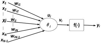
xj (j=1, 2, ...N) is input signal of neuron i, wij is connection weight, θi is threshold value of neuron, f is excitation function (also called action function), vi is output value in first layer after adjustment, and yi is output value of neural network. They are shown as the formulas (11-12) below:
(11)
(12)
f excitation function is consist of linear function, sesquilinear function and sigmoid function, and segmented function and others.
Learning algorithm of neural network requires good accuracy and convergence. Connection weights and threshold value obtain constant correction in learning process when using training samples for training. After this a better output (expected value) could be reached. The rules of learning algorithm are:
- Related rule: It denpens on excitation strength of connections between nodes to adjust network weights. And network weight correction formula (13) is based on Hebb learning rule where ui and uj are excitation values of node i and j respectively.
(13)
- Correction rule: It denpens on error between output value and expected value to correct network weights. δi is defined as output error of the node i, uj is excitation value of node j and η is learning efficiency.
(14)
- Non-tutor learning rule: There is an automatically adjustment adapted to network weights in learning process. The most basic one is Hebb learning rule, that is, if the neurons ui receives output value of another neuron uj, weight ωij from ui to uj is increased once both neurons get excited.
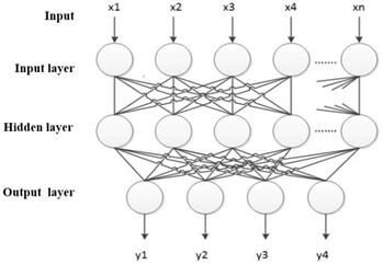
In other words BP neural network is the neural network with multi-layer feedforward, and error back propagation algorithm is its core learning ide. There are inter connection between input layer and hidden layer, hidden layer and each node of output layer. And the connection is one-way communication without any connection between neurons. Besides, its neuron function is S-type function. BP neural network corrects network weight and carry out training through gradient descent algorithm by which BP network output error could achieve the minimum effect. The BP network structure is shown in figure 4.
The structure of BP neural network
The BP algorithm can be described as below. At the beginning of the algorithm, the system will randomly select a network weight ranging between [-1,+1] to train for the purpose to reduce output er1ror. Then we use training set to train network where system will correct network weight if there is a great error between output value and expected output, and this is done through the back propagation algorithm. The error will slowly be converged and training process will make good or bad assessment on network through convergence speed. A certain network domain value and weight, which is the group with the smallest error between output and expected value, can be obtained by constantly modifying and substituting, and thus the optimal structure of the neural network is formed. The design of network structure and training samples is the two most important designs of BP neural network. Let's take a look at the design method:
Network data information capacity and training samples
The recognition ability is of tightness with its data information capacity. If Nω is used to represent network weight and threshold, then training sample number ρ and training error ε can be expressed by the following formula:
(15)
However practically training samples number could hardly achieve the requirement above. But Nω is proportional to input feature dimension. Therefore, it is known that characteristic vectors should be reduced when samples number is finite in order to reduce Nω.
Preparation (data acquisition and analysis and variable selection, etc.)
Selection and expression of outputs and inputs
Input is target signal characteristic and output is recognition target. In short, there are three kinds of recognition of lung sounds, so lung sounds category will display BP neural network output in the coding form.
Design of training set
The recognition performance is of tightness with its training set samples, so sample quality is of great significance. Besides, identified results can be more close to nature with more samples. However samples number is not the more the better. If samples number is too large, it would inevitably results in the decrease of recognition efficiency, so it is necessary to consider the actual situation under integrated balance between samples number and recognition efficiency. In algorithm we should cross the input with same kind of samples, so neural network can make mean for projection of all samples.
Initial weight and threshold values settings
It is needed to set initial network weight if you want to make transformation function of neurons in sensitive region, which improves speed of learning and convergence.
Structure design of BP neural network
Training samples can determine its layer nodes of input and output in target classification. Moreover, the normal actual classification problem generally adopts to neural network with three layers. It can be described on the number between input layer neurons N1 and hidden layer neurons N2 by the following formula:
(16)
Network training and test
Because training function is a kind of gradient descent algorithm, so it can be used for network training. Repeated corrections on weights and threshold could reduce error between final output value and expected value as far as possible. After completion of network training we can start with samples to test samples output values.
Simple structure and convenient operability is the advantage of BP neural network, although there are disadvantages such as slow learning convergence and that the network is very likely to fall into local minimum point. But these advantages do not affect that it is the most commonly used signals and the classification tool of image recognition. The error function can be obtained by formula (17) where i is the number of output categories and S is output value:
(17)
Wavelet decomposition and feature extraction
Wavelet decomposition
In the field of lung sounds research, there is no general large-scale database available. The data set used in this paper is from lung sounds database collected and constructed from the hospital. The lung sounds signal was collected by 3M Littmann digital electronic stethoscope with a sampling frequency of 4000 Hz. And lung sounds data were collected and analyzed by professional doctors. When collecting data, lung sounds data last for about 30 seconds could be collected. There are 64 typical cases of 6 normal lung sounds, 29 dry rales and 29 moist rales.
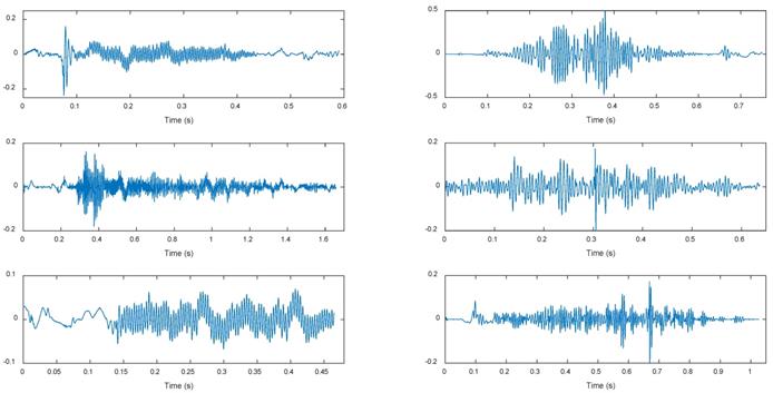
Both the references [39,40] below point out that the frequency both of dry rales and moist rales is higher than 100Hz. So we set the high-pass filter with the initial frequency of 100Hz to eliminate the noise which has lower frequency bands than the sound signals. However, the filtered signal still contains a part of heart sounds component and lung sounds and heart sounds are highly coincident in some frequency. Through threshold method [41], we use reconstructed signals obtained by wavelet transform to remove heart sounds interference, and get purer lung sounds signal reconstructed signals. And then we reconstruct wavelet signal for a purer lung sounds signal. Figure 5 shows waveforms of dry rales (left three groups) and moist rales (right three groups) after de-noising. It can be seen from figure that dry rales are more dispersed than moist rales. And dry rales' duration is longer and frequency is higher.
Waveforms of dry rales(left) and moist rales(right)
The frequency of lung sounds is mainly concentrated at 100~2000Hz [42]. According to sampling frequency of Nyquist sampling theorem, the sampling frequency of experimental signal is set as 4000Hz. It is observed that lung sounds signal frequency above 1000 Hz is scarcely ever so frequency needed to be analyzed could be set at 100~1000 Hz. In this paper, we use coif2 wavelet to decompose signal by five layers. The process is as follows: In the first decomposed layer, the initial signal frequency ranges from 0 to 2000Hz, and low frequency reconstructed signals A1 with 0~1000Hz frequency and high frequency reconstructed signals D1 with 1000~2000Hz frequency are obtained after decomposition. In the second decomposed layer, and low frequency reconstructed signals A2 with 0~500Hz frequency and high frequency reconstructed signals D2 with 500~1000Hz frequency are obtained after decomposition of the first layer. And so on, low-frequency reconstructed signals A5 with 0~63Hz frequency and high-frequency reconstructed signals D5 with 63~125Hz frequency are obtained by the fifth layer decomposition. In this situation, the frequency band is small enough for no longer decomposition. The frequency range of each layer is shown in Table 1 where Ai and Di denote low and high frequency band of layer i wavelet decomposition respectively. Table 2 shows the reconstructed signals frequency range after coif2 wavelet decomposition of five layers.
Reconstructed signals Frequency Range of five-layers Decomposition
| Layers number (i) | Ai | Di |
|---|---|---|
| 1 | 0~1000Hz | 1000~2000Hz |
| 2 | 0~500Hz | 500~1000Hz |
| 3 | 0~250Hz | 250~500Hz |
| 4 | 0~125Hz | 125~250Hz |
| 5 | 0~63Hz | 63~125Hz |
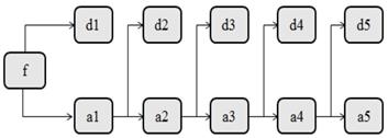
Low frequency part of wavelet decomposition signal in each layer is further decomposed into two parts of high frequency and low frequency parts, where high frequency part is no longer decomposed. Figure 6 shows wavelet decomposition construction of five layers.
Wavelet decomposition construction of five layers
For thresholds selection, there are various proposals for its choice including soft and hard thresholding, and thresholds that are fixed in advance or chosen level by level from an empirical optimality criterion [43]. For the consideration of that other methods may lose some information because of smooth de-noised signal, layered thresholds are selected as shown in formula (18).
(18)
In conjunction with soft threshold and Gaussian white noise, this threshold choice (VisuShrink) generally produces noise-free reconstructions [43], sometimes at cost of shrinkage of genuine features. After decomposition, lung sounds signals can be reconstructed by formula (19).
(19)
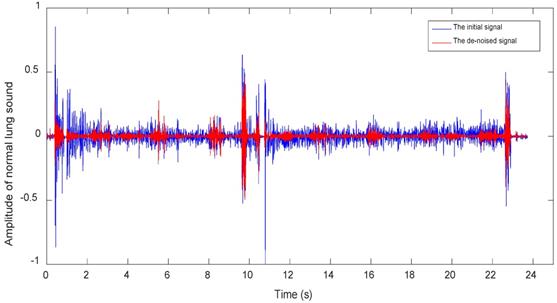
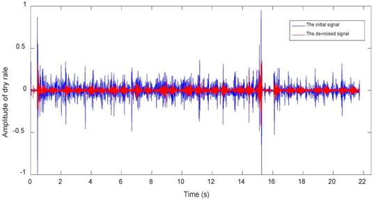
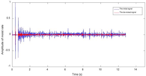
Figures 7~9 show waveforms of normal lung sounds, dry rales and moist rales before and after de-noising, where blue and red line represent signal curve before and after wavelet de-noising. Compared to signal before dealing (blue curve), the de-noised signal (red curve), which is relatively purer lung sounds, remove high-frequency details with 1000~2000Hz frequency and low-frequency approximations with 0~63Hz frequency.
Normal lung sounds waveforms before and after de-noising
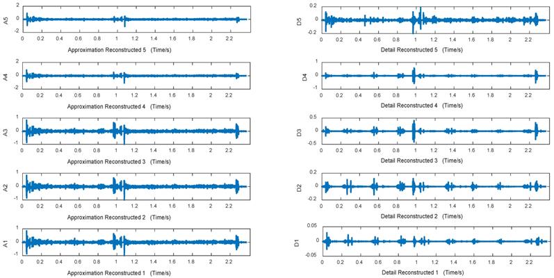
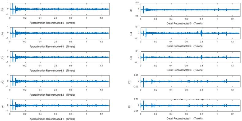
Figures 10~12 are approximation reconstructed signals and detail reconstructed signals in five layers from normal lung sounds, dry rales and moist rales. It can be seen that approximation detail reconstructed signals of dry rales signal exist sudden increase near the 1.6s, while reconstructed signals of moist rales exist sudden increase near the 0.8s.
Dry rale waveforms before and after de-noising
Moist rale waveforms before and after de-noising
Approximation and detail reconstructed signals in 5 layers of normal lung sounds
Feature extraction and linear discriminant method
The traditional sound features are mainly short-term energy, short-term average amplitude, zero-crossing rate, fundamental sound, etc., in which short-term energy, short-term average amplitude and zero-crossing rate are time-domain characteristics and fundamental sound is mainly used in sound recognition. With the development of sound classification and recognition, more sound characteristic parameters, which includes Linear Predictive Coding (LPC), Linear Predictive Cepstral Coding (LPCC), Linear Spectrum Pair (LSP), formant frequency, Mel frequency Cepstral Coefficents (MFCC) and its dynamic parameters, are more and more widely used in sound data analysis. In recent years, wavelet analysis has some applications in sound feature extraction, and sound feature extraction based on depth learning is also a hot topic in current research.
Normalized reconstructed wavelet energy
The original signal is decomposed and reconstructed to realize the separation of different frequency components. However, reconstructed signals are still high-dimensional data, and the reconstructed signals of different layers have different dimensions which cannot be used to directly represent signal characteristics.
Lung sounds of different types, which have different acoustic characteristics, should have different energy distributions over the entire frequency range. The normalized reconstructed signals are exactly the representation in specific frequency range of time domain signals. Therefore, reconstructed signals energy of each layer can be calculated as the frequency characteristic. The energy Ei corresponds to reconstructed signals Di of layer i shown in formula (20). And the normalized reconstructed signals energy is shown in formula (21).
(20)
(21)
Where n is the dimension of Di, m is the dimension of Ei,Di,j is the element j of Di, Ei is reconstructed signals energy and ENi is normalized reconstructed signals energy. EA1~EA5 represent normalized approximation energy of reconstructed signals of 1~5 layers, and ED1~ED5 represent normalized detail energy of reconstructed signals of 1~5 layers. Through these normalized energy values, 19 groups of normalized wavelet approximation and detail energy of sounds could be obtained.
Linear discriminant analysis
In order to reflect more essential data characteristics under the condition that eigenvectors are overmuch, we choose linear discriminant analysis to analyze 10-dimensional eigenvectors to find appropriate dimension for the effect of reducing space dimension. Linear discriminant analysis, which is to use the known category information to project training sample to the vector space that is most conducive to identification, could achieve the effect of simplifying spatial dimension. The training samples have minimum-in-cluster-distance and maximum-between-cluster-distance in the space after projection, that is different samples own the best separability in space.
Approximation and detail reconstructed signals in 5 layers of dry rale
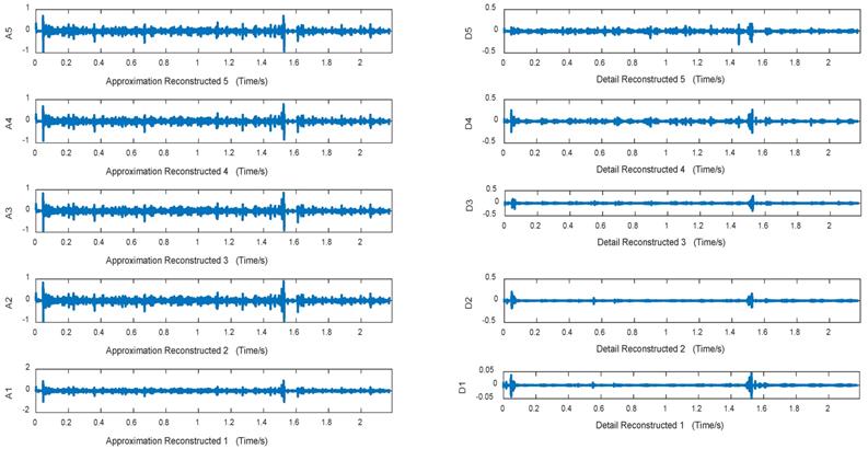
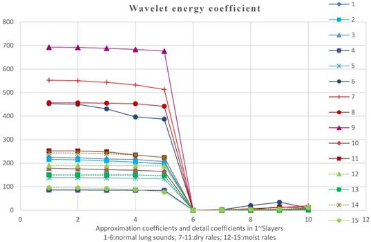
Figure 12 shows the reconstructed signals energy values which have not been normalized, that is, 10-dimensional characteristic parameters line graph of data of 19 groups. In this figure, the blue lines represent the normal lung sounds, black lines is on behalf of dry rales and red lines is on behalf of moist rales. These sounds are of some overlap in energy. Maybe it is because that the doctor gets some misjudgments when auscultating with data exported by 3M software or some other reasons. But most of the normal lung sounds energy are concentrated in 200~700Hz, dry rales are concentrated in 180~450Hz and moist rales are concentrated in 80-260Hz.
Approximation and detail reconstructed signals in 5 layers of moist rale
We used formula (21) to normalize the reconstructed signals energy corresponding to reconstructed signals energy values percentages. Then we use linear discriminant analysis to reduce dimension of previous 10-dimensional eigenvector by normalized typical function discriminant. And the following optimal four-dimensional eigenvectors are obtained: the approximation energy values 1 and 4 and the detail energy values 1 and 5. Table 3 is a linear discriminant optimal coefficients plot. Therefore, the analyzing data select EA1, EA2, EA5 and ED1 for further pattern recognition.
Optimal standardized coefficients of typical discriminant function
Function | Coefficient | Bootstrap | ||||
|---|---|---|---|---|---|---|
| Offset | Standardized error | Confidence interval of 95% | ||||
| Lower limit | Upper limit | |||||
| EA1 | 1 | 19.343 | -12.878 | 13.717 | -23.790 | 25.449 |
| 2 | -2.005 | -.316 | 7.175 | -21.021 | 11.878 | |
| EA2 | 1 | -18.841 | 9.243 | 12.957 | -25.545 | 19.584 |
| 2 | 1.637 | 1.683 | 7.244 | -9.776 | 22.574 | |
| EA5 | 1 | -.154 | .345 | 1.150 | -.529 | 3.052 |
| 2 | -.407 | .659 | 1.174 | -2.313 | 2.687 | |
| ED1 | 1 | .168 | -.171 | .310 | -.793 | .620 |
| 2 | 1.003 | -.447 | 1.004 | -1.209 | 2.504 | |
Experiment with BP neural network
With characteristic parameters after dimensionality deduction, the next pattern recognition and classification design of BP neural network can be carried on. Input values are set as 4 characteristic parameters, output values are set as 1~3 representing the normal lung sounds, dry rales and moist rales respectively. There are data of 64 groups where training data is 58 groups, conformed data is 3 groups and test data is 3 groups. Data distribution is random set inside neural network and data percentage can be adjusted. Figure 14 is values setting of BP neural network including data percentage distribution and number of hidden layers.
Reconstructed signals energy before normalized
Values setting of BP neural network
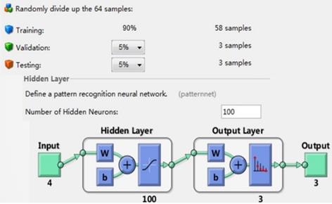
The number of training samples is 58 and the number of test samples and validation samples are both 3 (6 normal sounds groups, 29 dry rales groups and 29 moist rales groups). The hidden layers number is 100; learning rate is 0.1; allowable error is 0.01. While Yao et al. combined with wavelet analysis and genetic neural network method for statistical characteristic extraction and classifier design to distinguish lung sounds category whose recognition accuracy was 89% [27].
The recognition accuracy is determined by the average of more than 10 trainings. As for reconstructed signals energy data without LDA, the final recognition accuracy is 82.5% while the recognition accuracy of the data after LDA is higher as 92.5%. From this point, it can be concluded that the linear discrimination analysis shows its fine performance on dimensionality reduction of lung sound characteristic vector.
Conclusion
Combined with wavelet transform, linear discriminant analysis and BP neural network, we carry out multi-layers decomposition of lung sounds, and then it is well verified by lung sounds categories recognition with a recognition of 92.5% compared to the accuracy as 82.5% without LDA method.
Through wavelet transform, the analysis of lung sounds on frequency bands and different time positions is achieved. And we achieve the noise reduction of lung sounds with wavelet transform through which lung sounds are easier to be listened and distinguished by the professional doctors.
After linear discriminant analysis, we could achieve the dimensional deduction and data visualization under practical samples number. During this method, accuracy of training set sample characteristics and distribution will affect recognition results. It is a focus in future research on how to ensure that eigenvector contains more complete information of lung sounds before dimension reduction, and how to prevent the phenomenon of over-training and under-training.
The advantages of lung sound recognition through BP neural network are that training algorithm is relatively simple, and it is better to use reverse calculation of weight and fixed with gradient descent method. Through BP neural network, training learning speed is faster but the demand on samples is higher and it is easier to get into local small value. In addition, lung sounds recognition accuracy of our method as 92.5% is better than Yao et al.'s which is comparatively lower as 89%.
Acknowledgements
The research is funded by Grants (51575020) of the National Natural Science Foundation of China and Open Foundation of the State Key Laboratory of Fluid Power Transmission and Control.
Competing Interests
The authors have declared that no competing interest exists.
References
1. Guo R. China Ethnic Statistical Yearbook 2016. Springer International Publishing. 2017:227-248
2. Pauwels RA. GLOBAL STRATEGY FOR ASTHMA MANAGEMENT AND PREVENTION. Japanese Journal of Allergology. 2017;45:792-792
3. World Health Organization [WHO]. Global Observatory for eHealth. mHealth: New horizons for health through mobile technologies. Based on the findings of the Second Global Survey on eHealth. Geneva Switzerland Who. 2011:46-50
4. Semedo J. et al. Computerised Lung Auscultation-Sound Software. Enterprise Information Systems/international Conference on Project Management/conference on Health and Social Care Information Systems and Technologies. 2015;64:697-704
5. Shi Y, Wang Y, Cai M. et al. Study on the Aviation Oxygen Supply System Based on a Mechanical Ventilation Model. Chin. J. Aeronaut. 2018;31(1):197-204
6. Pokorski M. Respiratory System Diseases. Springer International Publishing. 2017:19-25
7. Ou D. et al. An electronic stethoscope for heart diseases based on micro-electro-mechanical-system microphone. IEEE, International Conference on Industrial Informatics IEEE. 2017;14:882-885
8. Daou RAZ. et al. A low-cost computerised electronic stethoscope with pre-diagnosis and easy transmission features. International Journal of Biomedical Engineering & Technology. 2017;23(1):38
9. Reynolds J. et al. Electronic Stethoscope With Wireless Communication to a Smart-phone, Including a Signal Filtering and Segmentation Algorithm of Digital Phonocardiography Signals. IFMBE Proceedings. 2017;60:553-554
10. Khan SI, Ahmed V. Investigation of some features for preliminary detection of coronary artery disease using electronic stethoscope. International Conference on Emerging Trends in Communication Technologies IEEE. 2017;24:1-3
11. Rosenthal RL. Electronic Stethoscope for Coronary Stenosis Detection. American Journal of Medicine. 2017;130(5):225
12. Huang M. et al. Computer-aided Diagnosis and New Electronic Stethoscope. Chinese Journal of Medical Instrumentation. 2017;41(3):161-161
13. Wang D. et al. The research progress about the intelligent recognition of lung sounds. IEEE International Conference on Computer and Communications IEEE. 2017;2:769-772
14. Riella RJ, Nohama P, Maia JM. Methodology for Automatic Classification of Adventitious Lung Sounds. Ifmbe Proceedings. 2009;25(4):1392-1395
15. Charleston-Villalobos S. et al. Assessment of multichannel lung sounds parameterization for two-class classification in interstitial lung disease patients. Computers in Biology & Medicine. 2011;41(7):473-474
16. Koulinas G, Kotsikas L, Anagnostopoulos K. A particle swarm optimization based hyper-heuristic algorithm for the classic resource constrained project scheduling problem. Information Sciences. 2014;277(2):680-693
17. Florence AP, Shanthi V. A load balancing model using firefly algorithm in cloud computing. Journal of Computer Science. 2014;10(7):1156-1165
18. Lu Q. et al. [Study for lung sound acquisition module based on ARM and Linux]. Chinese Journal of Medical Instrumentation. 2011;35(4):263-264
19. Hadjileontiadis H. Lung Sounds:An Advanced Signal Processing Perspective. 2008; 1: 100-103.
20. Shimoda T. et al. Lung sound analysis helps localize airway inflammation in patients with bronchial asthma. Journal of Asthma & Allergy. 2017;10:99-110
21. Shimoda T. et al. Lung Sound Analysis Is Useful for Monitoring Therapy in Patients With Bronchial Asthma. J Investig Allergol Clin Immunol. 2017;27(4):246-251
22. Xin XF. Advances in pulmonary sounds of pathology [J]. International Journal of Respiration. 1996;2:101-104
23. Hasse M. et al. Wheezes, crackles and rhonchi: simplifying description of lung sounds increases the agreement on their classification: a study of 12 physicians' classification of lung sounds from video recordings. Bmj Open Respir Res. 2016;3(1):136-140
24. Sun PL, Yin KS. Application of pulmonary sound map in diagnosis and treatment of respiratory diseases [J]. International Journal of Internal Medicine. 1999;10:436-438
25. Niu JL, Yan S, Cao ZX. et al. Study on air flow dynamic characteristic of mechanical ventilation of a lung simulator. Science China Technological Sciences. 2017;60(2):243-250
26. Ren S, Shi Y, Cai M. et al. Influence of secretion on airflow dynamics of mechanical ventilated respiratory system. IEEE/ACM Trans. Comput. Biol. Bioinform. 2017;99:1-1
27. Ren S, Cai M, Shi Y. et al. Influence of Bronchial Diameter Change on the airflow dynamics Based on a Pressure-controlled Ventilation System. Inter. J. Numer. Method. Biomed. Eng. 2017;34(3):569-573
28. Riella RJ, Nohama P, Maia JM. Methodology for Automatic Classification of Adventitious Lung Sounds. Ifmbe Proceedings. 2009;25(4):1392-1395
29. Yao XJ, Wang H, Liu S. Research on Recognition Algorithms of Lung Sounds Based on Genetic BP Neural Network. Space Medicine & Medical Engineering. 2016;12:334-340
30. Gurung A. et al. Computerized lung sound analysis as diagnostic aid for the detection of abnormal lung sounds: a systematic review and meta-analysis. Respiratory Medicine. 2011;105(9):1396-1403
31. Shi Y, Zhang B, Cai M. et al. Coupling Effect of Double Lungs on a VCV Ventilator with Automatic Secretion Clearance Function. IEEE/ACM Trans. Comput. Biol. Bioinform. 2017;99:1-1
32. Shi Y, Zhang B, Cai M. et al. Numerical Simulation of volume-controlled mechanical ventilated respiratory system with two different lungs. Int. J. Numer. Methods Biomed. Eng. 2016;33:2852-2859
33. Niu J, Shi Y, Cai M. et al. Detection of Sputum by Interpreting the Time-frequency Distribution of Respiratory Sound Signal Using Image Processing Techniques. Bioinformatics. 2018;34(5):820-825
34. Lee JS. et al. Anti-acid treatment and disease progression in idiopathic pulmonary fibrosis: an analysis of data from three randomised controlled trials. Lancet Respir Med. 2013;1(5):369-376
35. Zhao JH, Li WH. Intrusion Detection Based on BP Neural Network and Genetic Algorithm. Communications in Computer & Information Science. 2012;308(10):438-444
36. Niu J, Shi Y, Cai M. et al. Detection of Sputum by Interpreting the Time-frequency Distribution of Respiratory Sound Signal Using Image Processing Techniques.[J]. Bioinformatics. 2017;34(5):820-827
37. Shimoda T. et al. Lung Sound Analysis and Airway Inflammation in Bronchial Asthma. Journal of Allergy & Clinical Immunology in Practice. 2016;4(3):505-511
38. Sengupta N, Sahidullah M, Saha G. Lung sound classification using cepstral-based statistical features. Computers in Biology & Medicine. 2016;75:118-129
39. Serbes G. et al. Feature extraction using time-frequency/scale analysis and ensemble of feature sets for crackle detection. Engineering in Medicine and Biology Society, Embc, 2011 International Conference of the IEEE. 2011;2011:3314-3317
40. Hadjileontiadis LJ, Panas SM. A wavelet-based reduction of heart sound noise from lung sounds. International Journal of Medical Informatics. 1998;52(1-3):183-184
41. Donoho DL, Johnstone IM. Threshold selection for wavelet shrinkage of noisy data. Engineering in Medicine and Biology Society. Engineering Advances: New Opportunities for Biomedical Engineers. Proceedings of the, International Conference of the IEEE. 1994;1:A24-A25
42. Donoho DL. et al. Wavelet Shrinkage: Asymptopia? Journal of the Royal Statistical Society. 1995;57(2):301-369
43. Suboh A Z, Yaakop M, Yid M S M. et al. Segmentation of Heart Sound Signals into Cycles based on Peak Intervals Pattern[C]// International Conference on Engineering Technology & Technopreneuship. IEEE. 2015:301-304
Author contact
![]() Corresponding author: Email: yesoyoucom
Corresponding author: Email: yesoyoucom